To use incalead, you will have to install NetLogo 5.3.1 (free and open source) and download the model itself. Unzip the downloaded file and click on incalead.nlogo
InCaLead (Innovation, Catch-up and Leadership in Science-Based Industries) is an evolutionary model designed to explore the role of scientists' mobility, and the interactions among innovation, mobility and demand as key drivers of industrial leadership and catch-up. The model incorporates industrial scientists' training and migration, endogenous R&D decisions and the possibility of funding capital accumulation through debt.
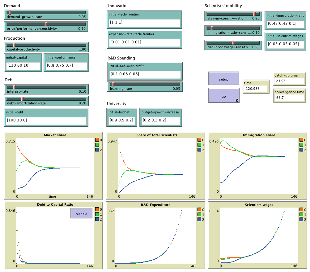
This section explains the formal model that InCaLead implements. The information provided here should suffice to re-implement the same formal model in any sophisticated enough modelling platform. We use bold red italicised arial font to denote parameters and initial conditions (i.e. variables that can be set by the user), and we use bold green italicised arial font to denote the name of the corresponding slider or box in the interface of the model above. All sliders can be changed at run-time with immediate effect on the dynamics of the model.
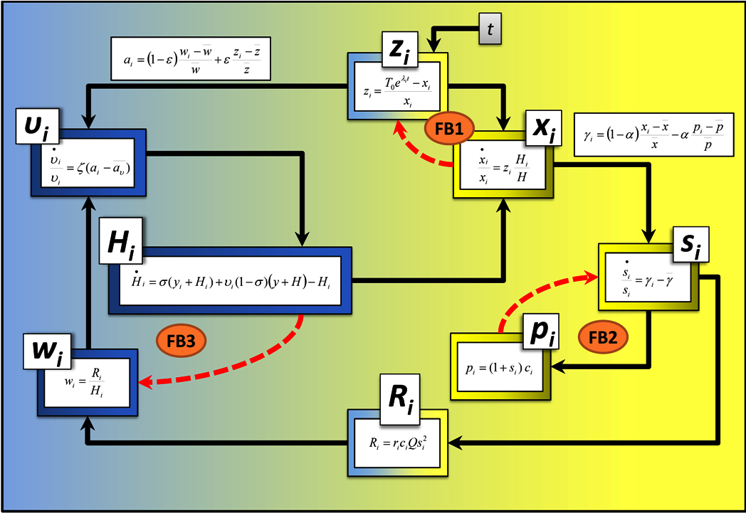
The figure below summarizes the main interactions among the most important variables in the model; it is a helpful reference to look at whilst reading the explanation of the model.
Sketch of the interactions among the most important variables in the model. The variables that are more closely related to scientists' mobility are represented towards the left, whilst the variables more related to the market for the product appear towards the right. These two subsystems affect each other in a number of ways. In fact, there are several negative feedback loops (red arrows) that favor the stability of various variables. For example, higher R&D productivities zi have a positive effect on performance xi, but this increase in performance diminishes the gap that separates the actual technological level from the technological frontier, and thus lowers R&D productivity (see FB1). Similarly, greater levels of competitiveness γi have a direct positive effect on market shares si, which lead to higher prices pi, which in turn imply lower competitiveness (see FB2). And finally, greater salaries wi attract mobile scientists, but this increase in the number of scientists Hi in a country puts pressure to lower salaries (see FB3).
In order to simplify the model's presentation, we classify our assumptions into five subsections: "The Firms' Competitiveness", "Demand Transformation", "Production and Growth", "Financing" and "Innovation and Institutions".
There are 3 firms, each one with a different national identity, competing at a worldwide level in a science-based sector. There is one firm per nation, so we can identify the representative firm of nation i with the i-th national industry. We assume that the firms compete over price pi and product performance xi (quality, reliability, size, speed, precision). Firms set prices applying a margin to the unit cost ci equal to their individual market-share si (larger margins for greater market powers). Thus,
pi = (1 + si)·ci
Thus, firm i's unit profit is
πi = pi - ci = si·ci
Regarding performance xi, we will establish below how firms improve their products through R&D-based technological innovations. For now, given the vector (pi, xi) we can define the level of competitiveness of firm i's product (as consumers perceive it in the global market) in the following way:
γi = (1-α)·(xi-x)/x - α·(pi-p)/p
where x = ∑jxj/3 and p = ∑jpj/3.
This formula captures the fact that consumers value both high levels of performance and low prices. The subjective relativity implied by the terms "high" and "low" is quantified using the average across the different products, whilst the trade-off between performance and price is regulated by parameter α (the price/performance-sensitivity of demand).
Production and growth are demand-driven. Regarding the demand-side of the market, we consider that the global demand (Qd) grows at a constant and exogenous rate g > 0 (demand-growth-rate), starting out from an initial level (Qd(0)). Likewise, as si is the proportion of global demand supplied by firm i -that is, its market share- we can see that the instantaneous demand of firm i will be:
Qdi = si·Qd = si·Qd(0)·egt
If we consider that the consumers interact among themselves, observing each other and disseminating information regarding prices and performances of different products, we can assume that there will be a gradual process of demand transformation. That is, consumers will withdraw their demand from certain firms and pass it on to others with a higher level of competitiveness γi. Drawing on Metcalfe (1998), we propose that this process of demand transformation can be represented by:
dsi/dt = si·(γi - γs)
where γs = ∑jsjγj.
Thus, the rate gdi at which demand for product i grows is:
gdi ≡ (dQdi/dt)/Qdi = g + (γi - γs)
It is then clear that those firms with higher than average levels of competitiveness will tend to capture a greater proportion of the demand, thus reaching above-average demand growth rates gdi.
Let us see how production and growth fit the evolution of demand. Starting out from a supply-demand equilibrium for each firm Qi(0) = Qdi(0) = Qsi(0), we assume that each firm's growth rate follows the growth rate of its demand. Hence, if we assume that all firms produce in accordance with technology, i.e.:
Qsi = A·Ki
where A > 0 is the capital-productivity, and Ki is firm i's capital, the following must be fulfilled:
gki ≡ (dKi/dt)/Ki = gsi ≡ (dQsi/dt)/Qsi = gdi = g + (γi - γs)
That is, the growth of physical capital Ki -and, therefore, of the output- in each firm fits the growth of its demand in such a way that, at all times, Qi = Qdi = Qsi is fulfilled. Moreover, it is clear that si = Qi / ∑jQj = Ki / ∑jKj
Once firms have covered their costs, they need to finance both their R&D activities and their investment in physical capital. Regarding R&D, we assume that firms finance these activities with current profits; that is to say, they do not resort to external financing for these expenses. Previous contributions in the literature (Greenwald and Stiglitz, 1990 or Chiao, 2002) associate this behavior with the uncertainty of R&D. To be specific, we assume that the firms devote a proportion ri ∈ (0,1) of their current profits to R&D, so that firm i's R&D spending is:
Ri = ri·πi·Qi
Clearly, ri is a firm-specific operating routine. According to Silverberg and Verspagen (2005), deciding the most convenient level of has traditionally been considered as an uncertain strategic choice. Therefore, instead of assuming that ri is calculated by applying any optimizing procedure, we will consider that firms adapt this routine by imitating the behavior of their most successful rival. More precisely, we will consider that firms update ri according to the following expression:
dri/dt = β·(r* - ri)
where r* denotes the R&D routine of the most profitable firm at the time, and β is the learning-rate.
Regarding physical investment, we assume that firms devote the necessary proportion of their current profits (free of R&D expenses) to finance the growth of Ki. That is, they finance it as much as possible with their own funds before resorting to debt for any remaining needs. This is seen in the following investment function:
dKi/dt = θi·(1 - ri)πi·Qi
Considering the previous equations, we obtain that θi is endogenously determined according to the following expression:
θi = (g + (dsi/dt)/si)) / ((1 - ri)πi·A)
This expression gives us the financial needs of firm i at any time. The following cases may occur:
This latter possibility leads us to introduce dynamics for the evolution of the firms' debts. If we assume that firms pay off their debts at a constant rate χ ∈ (0,1) (the debt-amortization-rate), we can see that the debt dynamics of each firm will be:
dDi/dt = MAX {0 , (θi - 1)·(1 - ri)πi·Qi)} - χi·Di
Finally, the total costs of each firm will include production costs and financial costs. If we denote the debt to capital ratio of each firm by di = Di/Ki, it is clear that firm 's unit cost will be
ci = (Ki + (η + χ)·Di) / Qi = (1 + (η + χ)·di) / A
Let us denote by Ti = Ti(0)·eλit the trajectory of the technological frontier of firm i. The initial technological frontier (Ti(0), the initial-tech-frontier) and its expansion rate (λi > 0, the expansion-rate-tech-frontier) determine the possibilities of innovation for firm i. It is well known (Freeman, 2004) that λi depends on the efficiency with which certain supporting institutions favor basic knowledge creation (national universities, public agencies and labs, industry-science interfaces, etc.).
Given this expanding frontier, we will assume, as in Nelson and Phelps (1966), that each firm innovates by exploring the gap separating its actual technological level (xi) from the technological frontier. This gap can be represented by zi = (Ti - xi)/xi. As in Nelson and Phelps (1966), we will assume that the rate of technological improvement is an increasing function of each firm/nation's human capital attainment, and proportional to the gap.
For formal convenience, we will measure each firm/nation's "human capital attainment" by the proportion (hi) of the overall stock of scientists working in the sector worldwide (H = ∑jHj) that each firm employs at any time; that is hi = Hi/H. Then, we can represent the rate of improvement in each firm product performance through the following (Nelson-Phelps type) innovation function:
(dxi/dt)/xi = zi·hi = ((Ti - xi)/xi)·hi
where zi can be identified with the productivity of R&D.
We will consider that Hi is determined by the supply and demand of scientists in each firm/national industry. Moreover, we assume that supply and demand fit instantaneously due to the flexible evolution of the scientific salary (wi) in each nation. If we consider that firms devote their R&D budgets to hiring scientists at a price given by the respective national scientific salary, the demand of scientists by firm i will be given by:
Hi = Ri / wi
The supply of scientists will come from two sources: firstly, those scientists trained by the i-th national university system that join the corresponding i-firm; secondly, those scientists that decide to migrate to firm i attracted by monetary and non-monetary considerations.
For the sake of simplicity we consider that the amount of scientists trained in disciplines relevant for the industry, who finalize their training in nation i at any time (yi), coincides with the volume of public resources (Bi) devoted to training in this discipline in the i-th national university system. If we assume that this university budget grows linearly, we obtain:
yi = Bi(0) + bit
where Bi(0) (the initial-budget) and bi (the budget-growth-increase) are parameters. It can be seen that both these policy parameters, as well as parameters Ti(0) and λi capture very important aspects related to the efficiency with which certain science-related supporting institutions function in different nations.
Regarding scientist mobility, we assume that there are two possibilities: remain in the same country (i.e. immobile scientists), or move (i.e. mobile scientists). At any point in time, a proportion σ ∈ [0,1] of the total amount of scientists are assumed to be immobile (σ is the stay-in-country-ratio), while the other (1-σ) constitute the pool of mobile scientists. Thus, if we denote by υi the share of the global stock of mobile scientists that join national industry i at any time, we can consider that υi changes depending on salary differences and the possibilities that scientists perceive to be able to carry out their work in different nations. We can associate the effectiveness of scientists' work in the different nations with the respective R&D productivity zi.Thus, we define the attractiveness ai of a country i as follows:
ai = (1-ε)·(wi-w)/w + ε·(zi-z)/z
where w = ∑jwj/3 and z = ∑jzj/3.
A nation/firm is perceived more attractive the higher the salaries it pays and the higher its R&D productivity. Like in the equation for the competitiveness, the subjective relativity implied by the term "higher" is modulated using the average across firms, whilst the trade-off between monetary and non-monetary considerations is regulated by the parameter ε, the r&d-prod/wage-sensitivity (which represents scientists' relative sensitivity to non-monetary considerations).
We model the movement of mobile scientists assuming that they will emigrate from their current country i only if there are other countries that are more attractive than theirs; when this is the case, they will emigrate from i to j at a rate proportional to the difference in attractiveness, i.e. a rate proportional to (aj - ai). These assumptions at the micro level give rise to the following equation at the macro level (see Fatas-Villafranca et al. (2009)):
(dυi/dt)/υi = ζ·(ai - aυ)
where aυ = ∑jυjaj.
where parameter ζ (the immigration-ratio-sensitivity) controls the sensitivity of the immigration ratio υi to differences in the attractiveness of each country. Thus, the equation above establishes that those firms from specific nations which pay scientists better, or which offer better conditions for developing their activities, will attract more mobile scientists than the others.
Assuming market clearing at any time, the following condition must be fulfilled:
dHi/dt = σ·(yi + Hi) + υi·(1-σ)·(∑jyj + ∑jHj) - Hi
Note that the first term in the right hand side of the equation above, i.e. σ·(yi + Hi), refers to the number of immobile scientists in country i at time (t + δt) when δt→0, whilst the second term, i.e. υi·(1-σ)·(∑jyj + ∑jHj), refers to the share of the total pool of mobile scientists that decide to emigrate to country i. We can then obtain the dynamics of the national scientific salary which guarantees market clearing as:
(dwi/dt)/wi = (dRi/dt)/Ri - (σ·(yi + Hi) + υi·(1-σ)·(∑jyj + ∑jHj) - Hi) / Hi
InCaLead is an evolutionary model of industrial catch-up which incorporates industrial scientists' training and migration, endogenous R&D decisions and the possibility of funding capital accumulation through debt.
Copyright (C) 2010 Isabel Almudí, Francisco Fatás-Villafranca & Luis R. Izquierdo
This program is free software; you can redistribute it and/or modify it under the terms of the GNU General Public License as published by the Free Software Foundation; either version 3 of the License, or (at your option) any later version.
This program is distributed in the hope that it will be useful, but WITHOUT ANY WARRANTY; without even the implied warranty of MERCHANTABILITY or FITNESS FOR A PARTICULAR PURPOSE. See the GNU General Public License for more details.
You can download a copy of the GNU General Public License by clicking here; you can also get a printed copy writing to the Free Software Foundation, Inc., 51 Franklin Street, Fifth Floor, Boston, MA 02110-1301, USA.
Contact information:
Luis R. Izquierdo
University of Burgos, Spain.
e-mail: lrizquierdo@ubu.es
This program has been designed by Isabel Almudí, Francisco Fatás-Villafranca & Luis R. Izquierdo, and implemented by Luis R. Izquierdo.